How to Categorize Queries for SEO Analysis via Python

Every query has different aspects in terms of entity profile, user, and search intent or its word counts. Thanks to queries (keywords or search terms), a Holistic SEO can understand how people think, what people care about, or what people fear, desire, or seek. According to the queries, the Search Engine Results Page (SERP) can be changed in terms of design and layout. Every web search activity, be it news search, image search, video search, or podcast search, begins with queries. People search the same things with different words and different things with the same words. That’s why disambiguation and search personalization along with SERP Designing, search intent classification is important. In this article, we will use Python and Mandy Wu’s Querycat Github Repo for the categorization of queries, after the categorization, we also will visualize the query clusters and use JR Oakles’ Google colab notes to perform this process.

What is Apriori Algorithm?

In this Guideline, we will use Apriori Algorithm via “Querycat”. Apriori Algorithm is created in 1994 by Rakesh Agrawal and Ramakrishnan Srikant. Apriori Algorithm’s purpose is that finding the similarities and common points between different data points in rows. It is useful especially for analyzing big data sets. Today, an e-commerce shop can find common points of different products in terms of purchase processes thanks to the Apriori Algorithm. Since the discovery of products that can be sold together will be possible, the product suggestion system can be improved.

In the Apriori Algorithm, there are four types of association rules. Learning these rules will help us to understand how and with what methodology we will categorize our queries.

Apriori Algorithm association measure methodologies:

• Support: It shows how different items can be found together in a data set. For instance, in the sentence “You should pick up those apples from the floor”, every word has been used only once, and also they are being used together only once. In the next sentence, “No, I won’t pick up those apples from the floor”, every word has been used once but also we have repeated some word groups such as “from the floor”. So, we may conclude that in this brief paragraph “from the floor” item set can occur more frequently than others. The same logic goes with also the Apriori Algorithm. If a person buys an apple with a beer, this will give +1 possibility point for co-occurrence in e-commerce behavior.
• Confidence: It calculates the likelihood of happening the co-occurrence. Let’s say a person buys 100 apples but zero beers. The second person buys 50 Apples and also 100 beers. So, in this example, we need to divide the number of “apple sales without beer” and “beer sales with apples”. So, our confidence for co-occurrence will be increased in logic.
• Lift: In this example, we also strengthen our logical conclusion. We divide the number of co-occurrence for both items in sales to the same items’ solely sales numbers’ multiplication. For instance, in a shop, let’s say 100 beers sold without any apple and 100 apples sold without any beers, also 500 apples and 500 beers are sold together in the same shopping activity. So, our Lift Score is 500/100×100, if the result is under the 1 it means that there is no co-occurrence, if it above the 1, it will mean that there is a correlation between these two items’ sales activities.

In our guide, we will use Querycat in our local machines, not in Google colab, but if you want you may use it via Google Colab by researching JR Oakles’ Github Repo (Source: https://github.com/jroakes/querycat/blob/master/Demo.ipynb)

To learn more about Python SEO, you may read the related guidelines:

1. How to resize images in bulk with Python
2. How to perform TF-IDF Analysis with Python
3. How to crawl and analyze a Website via Python
4. How to perform text analysis via Python
5. How to test a robots.txt file via Python
6. How to Compare and Analyse Robots.txt File via Python
7. How to Categorize URL Parameters and Queries via Python?
8. How to Perform a Content Structure Analysis via Python and Sitemaps
9. How to Check Grammar and Language Errors with Python
10. How to use Google Trends via Python for SEO?
11. How to scrape People Also Ask for Questions from Google via Python
12. How to check Status Codes of URLs in a Sitemap via Python

What is FP Growth Algorithm

The FP Growth Algorithm is a similar algorithm to the Apriori, it is also used for finding frequent patterns in datasets. It compresses the dataset and creates an “FP Tree” instance, then it divides the “FP Tree” according to their groups and turns all of the different databases, lastly, it processes all of those datasets at the same time. So, in short, it does the same thing in a shorter time. In this guideline, we have used the Apriori Algorithm first, but in the future, we will update this guideline with new methodologies.

What is Querycat and How to Download it?

Querycat is a small Python module for the classification of queries according to the word frequencies and co-occurrence levels of words (Source: https://github.com/mandywu/querycat). To use Querycat, we will download it into our computer system. You may follow the visual below to download it.

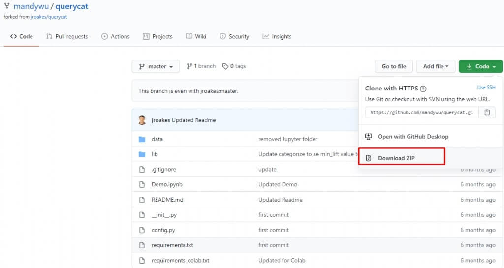
After the download is completed, you should extract the “zip file” and open your CMD. You should enter into the extracted file’s path via “cd” command in CMD and write the command below:

pip install -r requirements.txt

You may see the output below:

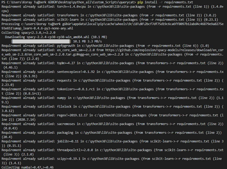
In every Requirements.txt file, there are dependencies for the library’s itself so that it can work with the necessary modules. We have downloaded all of the dependencies with single line of code. You may also use “!git” and “!pip” commands in Jupyter Notebook so that you can download them via Github as below:

!git clone https://github.com/jroakes/querycat.git
!pip install -r querycat/requirements.txt

You may see the output below:

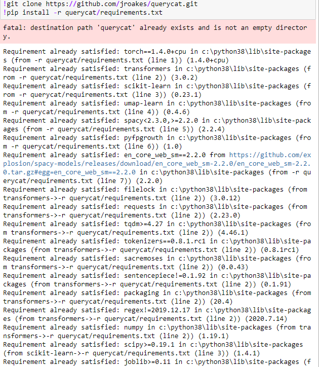
Since, we have already downloaded them, computer system says that “requirement already satisfied”.

Now, we may import “querycat”.

import querycat

You may see the output below:

What is NLTK Data?

The NLTK Data or Natural Language Toolkit Data is a program for building Python Scripts via Human Language. It is built by Steven Bird, Edward Loper and Ewan Klein. NLTK includes text-parsing, tokenization, classification, semantic reasoning and structuring libraries. When we import the “querycat” it starts to update “nltk_data” libraries so that everything can work smoothly.

How to Use Querycat?

The Querycat python package uses the Pandas Library for creating data frames. I have download the May and April Traffic Comparison Data for a web entity that lost the May 6th Core Algorithm Update. My purpose is to see that in which query group, the organic traffic loss happened most.

df = querycat.pd.read_csv('Queries.csv')
df.head(20)

We have turned our CSV file into a dataframe with “df” variable and called the 20 lines from the top.

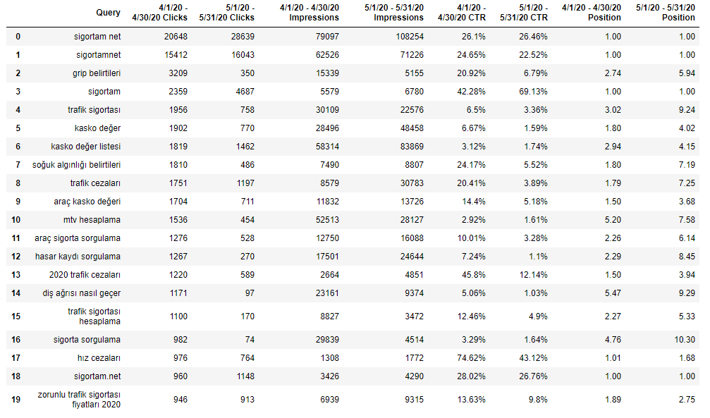
In the next line, I will change the names of the columns.

df.rename(columns={'Query': 'query', '4/1/20 - 4/30/20 Clicks': 'April Click','5/1/20 - 5/31/20 Clicks':'May Clicks', '4/1/20 - 4/30/20 Impressions':'April Impression', '5/1/20 - 5/31/20 Impressions': 'May Impression','4/1/20 - 4/30/20 CTR': 'April CTR', '5/1/20 - 5/31/20 CTR':'May CTR', '4/1/20 - 4/30/20 Position':'April Position', '5/1/20 - 5/31/20 Position':'May Position' }, inplace=True)

Now, we can start to categorize our queries with Querycat and Apriori Algorithm.

query_cat = querycat.Categorize(df, 'query', min_support=10, alg='apriori')
OUTPUT>>>
Converting to transactions.
Normalizing the keyword corpus.
Total queries: 1352
Total unique queries: 1220
Total transactions: 1219
Running Apriori
Making Categories
Total Categories: 122

The “querycat.Categorize()” method takes 6 attributes at most. These are “position” which is for specifying the data frame for categorization, “col” which is for specifying the column to be used for categorization, “alg” is for specifying the algorithm which we will use for categorization, it can be “Apriori” or “FP Growth Algorithm”, “min_support” is for the determining the minimum level of co-occurrence level for being counted as grouped, “min_probability is for finding the patterns for associated items with only “FP Growth Algorithm” and “min_lift” is for finding the associated word patterns with only the Apriori Algorithm.

In our output, we see that with at least 10 co-occurrence “minimum support” and “apriori” algorithm, we have 122 Query Categories over 1220 unique queries. Querycat inserts these categories and their “perception way” into the columns in our data frame. We may check the latest version of our data frame.

df.head(20)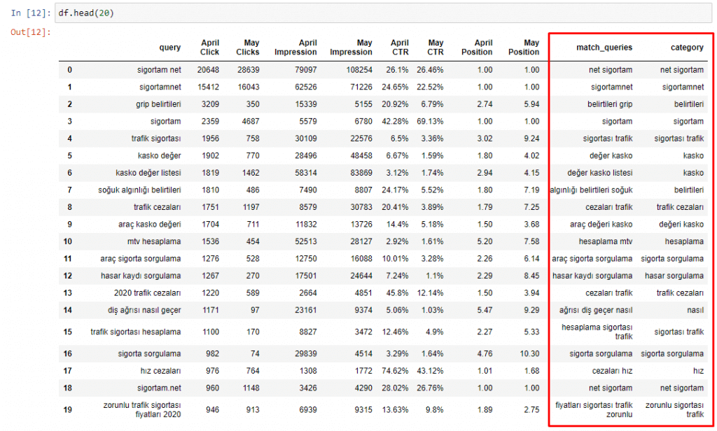

You may see that we have two new columns, one for “match queries” and other one for the “category” of the query. Match Queries show the matching part of the query for the specific query category. For instance for the “hız cezaları” we see that it uses the “cezaları hız” (speed penalties) for matching and put it into the “hız” (speed) category. But still, I can’t say that this is a right decision, I would prefer it in the “cezaları” (penalties) category. So, you may need to change your code via attributes or source code so that you can create more optimized queries. Also, you may get better results in different languages.

We may see which category have how many queries with Pandas’ “count()” method.

query_cat.counts.head(20)

You may see the output below:

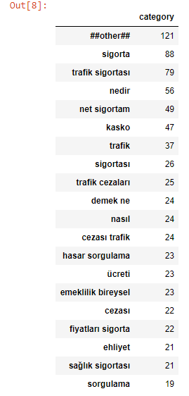
The other section is the ones that can’t be categorized according to our dataset’s language, our algorithm and min_support values. Also, in repeated requests, your data slightly differentiate. The other sections actually give hints about the query groups’ intents and their topics. We also may show the difference of click or impression data between May and April for those categories with Pandas Methods:

query_table = query_cat.df
query_table = query_table.groupby(['category'], as_index=False).agg({'query':'count', 'April Clicks':'sum', 'May Clicks':'sum'})
query_table['Difference'] = query_table['May Clicks'] - query_table['April Clicks']
query_table.sort_values(by='Difference', ascending=True, inplace=True)
query_table.head(20)

• The first line is for assigning our “Categorize Object” into a variable.
• The second line is for grouping the data frame according to the “category” column, “as_index=False” is for holding the index numbers in the output.
• “agg()” method is for aggregating our data columns, simply we want “sum” of values from two columns along with data count from another column.
• At the fourth line, we are creating a new column with the name of “Difference” so that we can see the click count difference between two months.
• We are sorting our data frame at the fifth line according to the values on the “Difference” column in ascending order.
• We use the “inplace=True” attribute for changing our data frame as permanently and calling the top 20 lines.

You may see the output below:

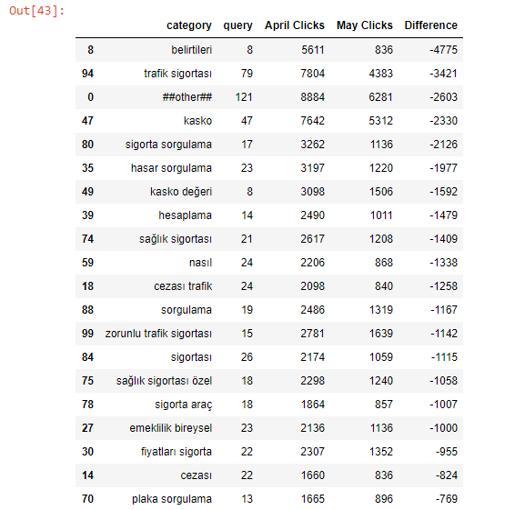
We see that our “belirtileri” (symptoms) category has 9 queries and they have lost more than 4000 clicks after the May 6th Core Algorithm Update. This category groups are actually about “disease symptoms”, an insurance aggregator brand has lots of articles about diseases and their treatment, so Google has decided to devalued these pages. When I have checked these pages, I have seen that the pages don’t have enough expertise and also they are about different Knowledge Domain, they even didn’t talk about “health insurance” or anything related to the “insurance”. So Google may decide to devalue all of those kinds of content. If you write something out of your Knowledge Domain, you should create a relevance so that Google Algorithms may see that this content create value for your users and target market, also try to create health content with high expertise. So, I have concluded these after this quick check-up. Also, “Trafik Sigortası” (traffic insurance) lost more than 3000 clicks. We may do this also with Average Position, CTR, and Impression Data to see the correlation between GSC Data.

We may reverse the data frame with changing “ascending=True” into the “ascending=False”.

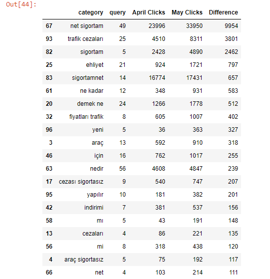
And we see that the Brand’s search demand has been increased after the Core Algorithm of May and its effects. This can happen because of the rankings lost, if users can’t see the brand on the SERP, they can search for it with the brand name. Or, this can happen because of a seasonal campaign. We need to see the Brand’s Search Terms and Latest Related Topics and Rising Keywords to see these. For this kind of situation, you should use PyTrend, and you can read our “Pulling Search Trends on Google via PyTrends” guideline. Now, we will focus on visualizing the click change according to the queries and using BERT (Bidirectional Encoder Representations from Transformers) Algorithm via Querycat for finding the queries’ similarity level in the categories.

With a single line of code, we can process our queries and put them into embeddings. Querycat has a special class called BERTSim(). It finds the similarity between the terms. Before proceeding, you should open the Querycat Folder in your Python environment and change the “TRANSFORMER_MODEL”. Querycat uses the distilbert-base-uncased model. According to your language, you should choose another model. Distilbert-base-uncased Model is an NLP Model from “Huggingface Transformers Repo” (Source: https://github.com/huggingface/transformers).

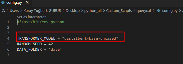
For our guideline, I didn’t change it. We may continue for finding the similarity level between our queries.

BERTSim() method has 3 different functions, these are “read_df” for reading the data frame, “get_similar_df” is for finding the most similar category with the given term, “diff_plot” is for plotting the differences in 2d vectors with “umap”, “pca” and “tsne” algorithms.

First, we will turn our data frame into a BERTSim() class.

bert_similarity = querycat.BERTSim()
bert_similarity.read_df(query_table, term_col = 'category', diff_col = 'Difference')

We have assigned the “querycat.BERTSim()” into a variable to use the functions we talked about above. Then, we have used the “read_df” function with our “query_table” data frame based on our “category” column to look at words and we have used the “diff_col” attribute to calculate differences between selected columns. We will use “get_similar_df” method below:

df_similarity = bert_similarity.get_similar_df('kaza')
df_similarity.sort_values(by='sim', ascending=False, inplace=True)
df_similarity.head(20)

The first line is for assigning the “get_similar_df” method into a variable and we have chosen the “kaza”(accident) string as our word.
The second line is for sorting the values according to the “sim” column, in descending way as permanent.
The third line is for getting the top 20 lines from our data frame.

You may see the results below:

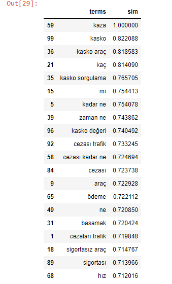
It says that the “kaza”, “kasko” and “kasko araç” query groups have the most similar queries in our given query which is again “kaza”. “KASKO” is the name of “Traffic Accident Insurance”, “KASKO Araç” is equilevant of “Traffic Accident Insurance for Cars”. Let’s change our query so we may see how the groups and similarities will change.

df_similarity = bert_similarity.get_similar_df('sağlık')
df_similarity.sort_values(by='sim', ascending=False, inplace=True)
df_similarity.head(20)

“sağlık” means “health”. “Sigortası sağlık”, “Sigortası özel sağlık” means “Health Insurance” and “Private Health Insurance” . As you may see below, they have the highest similarity.

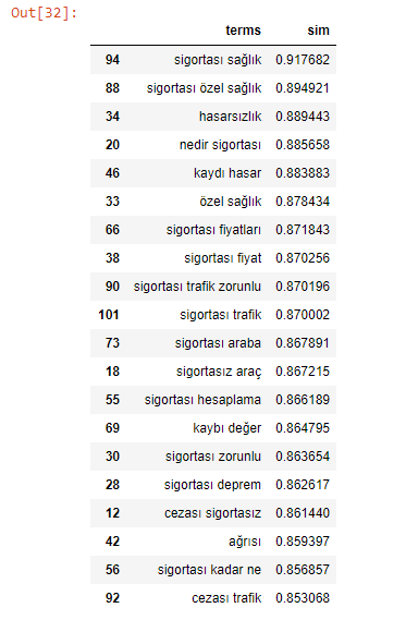
Why is finding these similarities are useful? You may quickly pull the necessary category groups for a specific query or intent thanks to “querycat.BERTSim()” class. Also, it will help you to see unnecessarily identical query category groups so that you can unify them later or you may pull the necessary data in a more comprehensive way.

Now, we will use the “diff_plot” for plotting the click change for specific query categories.

bert_similarity.diff_plot(reduction='umap')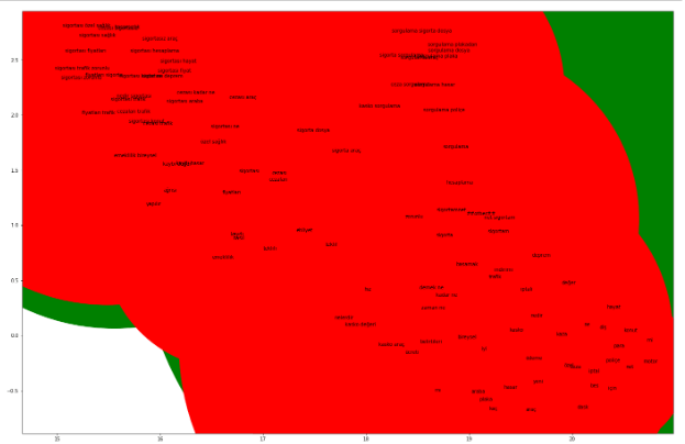

You may also use the “tsne” or “pca” algorithms for visualization. In this example, most of the visualization is green because of the “diff_col=’Difference'” attribute in our “read_df” method. Green shows the positive change in click amount unlike red, also the size of the bubble shows the difference magnitude. Every query group on the map is placed according to their relevance and similarity between them. This simple method (diff_plot()) is an opportunity to see general change according to the query intents. You may also use matplotlib or plotly for visualization by yourself for a better comprehension, if you want.

Query Classification with Python and Its Importance For SEO

Query classification based on search intent and grouping the queries according to their relevance by analyzing the organic traffic performance is an important improvement for SEO. You may categorize the queries even with Google Sheets, Javascript but plotting them and manipulating the data frames or using AI Algorithms on them is way much easier with Python. Query classification and intent classification for queries will be more relevant for SEO in the future. Without understanding the intent, a web page may not perform its purpose and due to this, it can lose ranks.

Our guideline is based on JR Oakles’ Google Colab and Mandywu’s Github Repo for now, but by the time we will expand this guideline with the new techniques for Holistic SEOs.

• Author
• Recent Posts

Koray Tuğberk GÜBÜR

Owner and Founder at Holistic SEO & Digital

Koray Tuğberk GÜBÜR is the CEO and Founder of Holistic SEO & Digital where he provides SEO Consultancy, Web Development, Data Science, Web Design, and Search Engine Optimization services with strategic leadership for the agency’s SEO Client Projects. Koray Tuğberk GÜBÜR performs SEO A/B Tests regularly to understand the Google, Microsoft Bing, and Yandex like search engines’ algorithms, and internal agenda. Koray uses Data Science to understand the custom click curves and baby search engine algorithms’ decision trees. Tuğberk used many websites for writing different SEO Case Studies. He published more than 10 SEO Case Studies with 20+ websites to explain the search engines. Koray Tuğberk started his SEO Career in 2015 in the casino industry and moved into the white-hat SEO industry. Koray worked with more than 700 companies for their SEO Projects since 2015. Koray used SEO to improve the user experience, and conversion rate along with brand awareness of the online businesses from different verticals such as retail, e-commerce, affiliate, and b2b, or b2c websites. He enjoys examining websites, algorithms, and search engines.

Latest posts by Koray Tuğberk GÜBÜR (see all)

• Sliding Window - August 12, 2024
• B2P Marketing: How it Works, Benefits, and Strategies - April 26, 2024
• SEO for Casino Websites: A SEO Case Study for the Bet and Gamble Industry - February 5, 2024